GPT2 from Scratch Part 2

Part 2 - GPT2 from Scratch: Attention Mechanism and Transformer

Table of Contents:

1. Embedding Layer
   1. Word Embedding
   2. Positional Embedding
2. Attention Layer
   1. Motivation for Attention
   2. Scaled Dot Product Attention
   3. Causal Self Attention
   4. Multi-head Self Attention
   5. PyTorch’s Attention Layer
3. Transformer Layer
   1. Layer Normalization
   2. GELU Activation
   3. MLP Layer
   4. Residual Connection
4. GPT Model
   1. Model Architecture
   2. Generate Text
   3. Greedy Decoding
   4. Top-K Decoding
   5. Effect of Temperature

Prerequisites

• Firstly, a medium level knowledge of Python (including OOPs concepts) is required, as the implementation will be carried out in this language.

• A foundation level machine learning concepts is needed to understand the concepts. This includes neural networks, loss functions, training dynamics etc. The knowledge of Recurrent Neural Network (RNN) is a bonus but not strictly needed.

• Experience with deep learning frameworks PyTorch is necessary, as it will be used to build and train the model. Basic knowledge of Huggingface library is a plus.

• A basic mathematical background in linear algebra and probability will support the understanding of model operations.

Previous Blog

In Part 1 of this blog, I have covered the aspects of data preparation process for GPT model which includes basics of embedding, tokenization process and sliding window method of data sampling.

1. Embedding Layer

1.1. Word Embedding

1.2. Positional Embedding

1.2.1. Why is “Position” Important?

We have already seen the word embedding which converts the integer token IDs into a continuous finite dimensional real vector representation. In Section 3.1: Working Principle of GPT, I have explained in detail that a GPT model processes an entire token sequence in one time step which is fundamentally different from an RNN model which processes a token sequence one at a time step which makes these models to compute the outputs “recurrently”. In summary, RNN process one token at a time which means that the positional information of the tokens are implicitly considered in the computation due to the nature of “recurrence” computation in RNN models. Since it handles the tokens one at a time, it knows which token appears first and which token appears last in the sequence as the position of token and time step of processing that token are exactly identical.

Tokens: ["I", "love", "machine", "learning"]
Positions: [0, 1, 2, 3]
Time Step: [0, 1, 2, 3]

In contrary, the GPT models perform its computation in such a way that it doesn’t need to know the tokens one by one in steps, rather it has the capability of computing all the tokens, all at one time step, therefore removing the “recurrence” component from the model. This improves the time complexity of the computation significantly as compared to RNN model. Although, in search of improving the computational cost, we “lost” one important aspects of RNN model - implicit positional information.

Since, the GPT models process the entire sequence using a mechanism called attention which doesn’t have any notion of “position” or “order” of the tokens in the sequence (as it processes the tokens all at one time step using linear combination of embedding vectors), the model has no way to figure it out the positional information from the sequence. I will revisit this point again in next section where I will talk about the attention mechanism.

For those who cannot wait to know the reason, I am going to provide a brief intuitive explanation for this. You can think the attention mechanism as a function which takes the embeddings of all the tokens as an input and returns the contextual embedding vector of all the tokens as an output. At its core, this function computes or “attends” all the input embedding vectors by taking the similarity (or dot product) with all the other vectors. It means the attention mechanism can be though of taking the linear combination of all the input embedding vectors at a token position where the combination coefficient will vary as we move from one token position to another token position during the computation of context vectors. Think the combination coefficients as a measure of the relevance or importance of each token in the sequence relative to the current token.

[ \mathbf{c}^k = \sum_{i = 1}^{T} \alpha _i^k \cdot \mathbf{x} _i \quad (\forall k \in {1, 2, \dots, T}) ]

Where $\mathbf{x} _i$ is the input embedding vector and $\mathbf{c}^k$ is the $k$-th output context vector. The combination coefficient (often called attention weights) are permutation invariant which means if we provide the sequence $(\mathbf{x} _1, \mathbf{x} _3, \mathbf{x} _2)$ instead of $(\mathbf{x} _1, \mathbf{x} _2, \mathbf{x} _3)$ then the attention weights will be readjusted accordingly by the attention function automatically (which is kind of a black-box to us at this moment) to produce the same output context vector. For instance, whether a sentence starts with “Variable x is pointer array” or “Variable x is array pointer”, the model recalibrates the attention weights to maintain contextually appropriate output vectors. That is why the order of tokens in a sequence does not matter to the attention function!

Consider a hypothetical vocabulary of only 5 tokens and each of the tokens are embedded by a 3 dimensional vector. Therefore, the token IDs can be either 0, 1, 2, 3, 4. Let’s take two possible sequence of token IDs as follows:

E = [[0.1, 0.2, 0.3, 0.4, 0.5],
     [0.6, 0.7, 0.8, 0.9, 1.0],
     [1.1, 1.2, 1.3, 1.4, 1.5]] # Embedding Matrix size is (d, V)

token_IDs_A = [1, 2] # (x1, x2)
word_embedding_A = [[0.2, 0.7, 1.2], 
                    [0.3, 0.8, 1.3]] # Extracts 1-st and 2-nd column from E
token_IDs_B = [2, 1] # (x2, x1)
word_embedding_B = [[0.3, 0.8. 1.3],
                    [0.2, 0.7, 1.2]] # Extracts 2-nd and 1-st column from E

Note that when we are changing the order of tokens in a sequence, the embedding vectors $\mathbf{x}$ values are not changed! It is only the position of the vectors that are changed. From the previous section, it is obvious that the embedding vectors are nothing but the columns of the embedding matrix. The embedding vector for a token ID is found after extracting its corresponding column from the embedding matrix. Therefore, the order in which the columns are extracted is changed but the individual column elements ($d$ elements in each column) are not changed! Therefore, the attention computation is not affected as the attention weights will just be readjusted. For example, $\mathbf{c} = \alpha _1 \cdot \mathbf{x} _1 + \alpha _2 \cdot \mathbf{x} _2 + \alpha _3 \cdot \mathbf{x} _3$ when the sequence is $(\mathbf{x} _1, \mathbf{x} _2, \mathbf{x} _3)$ which is same as $\mathbf{c} = \alpha _1’ \cdot \mathbf{x} _1 + \alpha _2’ \cdot \mathbf{x} _3 + \alpha _3’ \cdot \mathbf{x} _2$ when the sequence is $(\mathbf{x} _1, \mathbf{x} _3, \mathbf{x} _2)$. Note these two linear combinations are exactly same. It is just the readjustment of the attention weights ($\alpha _1’ \leftarrow \alpha _1, \alpha_2’ \leftarrow \alpha _3$ and $\alpha _3’ \leftarrow \alpha _2$) that makes it permutation invariant. You can also think it as a consequence of the fact that the vector addition in a vector space $\mathbb{V}$ which is denoted as $+ _\mathbb{V}$ or simply $+$ (when the context of $\mathbb{V}$ is clear then the subscript can be removed) is a commutative operator.

If you have not understood this above section on attention, it’s absolutely fine as it will be more clear when I will unwrap this attention “black-box” in the next section.

Let’s first understand why the position or order of tokens in a sequence matter in natural language. Consider the following two sentences:

Sequence 1: "Although, I did not understand the Attention mechanism, I was engaged with the blog!"
Sequence 2: "Although, I did understand the Attention mechanism, I was not engaged with the blog!"

If you tokenize these two sequences, it will give you the exact same tokens, but in different order. If we do not consider the order of the tokens in a sequence, then the above two sequences will possess same meaning. Although, in reality, it is not the case! These two sentences are clearly contradictory of each other in literal meaning. Therefore, it’s established that the position of the token in a sequence is the most important property of the sequence which needs to be captured by the GPT model. Since there is no direct way to capture it implicitly, we need to “inject” some positional information to the model explicitly so that it can understand the text better as “position” is what makes a sequence to behave like “text sentence”.

The positional embedding is also a vector in the embedding space which has the same dimension as the word embedding space. Therefore, at the token position $i$, to get the final embedding input vector ($\mathbf{t} _i$), we will add the word embedding vector ($\mathbf{x} _i$) and the positional embedding vector ($\mathbf{e} _i$) element-wise.

[ \mathbf{t} _i = \mathbf{x} _i + \mathbf{e} _i \quad \in \mathbb{R}^d ]

1.2.2. Properties of Positional Embedding

Before I talk about the properties of a “good” positional embedding, let’s first take a couple of examples of what constitutes a “bad” positional embedding.

Since we are interested to encode the positions of each tokens, as a naive approach, one could propose of using just the sequence numbers as their representation of positions. Mathematically, we can have a position embedding of a token at position $i$ such that:

[ \mathbf{e} _i = (i) _{j=0}^{j=d-1} \quad \text{in other words,}\quad e _i^j = i \quad \forall j = {0, 1, \dots, d-1} ]

For example if we have an embedding dimension of $d=5$ and a sequence of $T=1024$ tokens then:

x0 = [0.1, 0.05, 0.14, 0.42, 0.25] # Word embedding at token position 0
e0 = [0, 0, 0, 0, 0] # Position embedding at token position 0

x1 = [0.16, 0.72, 0.28, 0.39, 1.5] # Word embedding at token position 1
e1 = [1, 1, 1, 1, 1] # Position embedding at token position 1

...

x1023 = [0.19, 0.72, 0.93, 0.44, 0.51] # Word embedding at token position 1023
e1023 = [1023, 1023, 1023, 1023, 1023] # Position embedding at token position 1023

But will this “naive” positional embedding work in real life applications? Of course, it wouldn’t work. Ultimately, we are going to add the word embedding vector and the positional embedding vector element-wise. Therefore, for long sequences, the final input embedding will be completely governed by the positional embedding alone. For example, the addition of x1023 and e1023 will be approximately equal to e1023. This means, we have lost the information of “words” in the sequence, and it only captures the positional information of the sequence. As a result, the language model trained on this “naive” positional embedding is bound to fail in real life applications. From this “bad” positional embedding, we have identified one important property of a “good” positional embedding as follows:

Property 1: The positional embedding should be designed in such a way that there is a fair amount of balance between the word information and the position information. In other words, the positional information should not dominate fully in the input embedding.

One could think to improve the above positional embedding by “normalizing” it. It means, we are going to rescale the absolute sequence numbers to lie in between [0,1] by dividing it to the largest sequence number. In this way, we will make sure that all the positional embedding values are in between [0,1]. Therefore, if there are $T$ tokens, then we will divide each position index (absolute position in the sequence) by $T-1$.

For example if we have an embedding dimension of $d=5$ and a sequence of $T=1024$ tokens then:

x0 = [0.1, 0.05, 0.14, 0.42, 0.25] # Word embedding at token position 0
e0 = [0, 0, 0, 0, 0] # Position embedding at token position 0

x1 = [0.16, 0.72, 0.28, 0.39, 1.5] # Word embedding at token position 1
e1 = [1/1023, 1/1023, 1/1023, 1/1023, 1/1023] # Position embedding at token position 1

...

x1023 = [0.19, 0.72, 0.93, 0.44, 0.51] # Word embedding at token position 1023
e1023 = [1, 1, 1, 1, 1] # Position embedding at token position 1023

Again, a natural question would be: will this positional embedding work? The answer would be “no”. In this normalization process, we are making the positional embedding as a function of sequence length $T$. This means, if the model sees two sequences of two different lengths, then for the same position, there will be two different positional embedding. This violates the fundamental property of any positional embedding which says the positional embedding should be entirely dependent of position and not the sequence length.

For example if we have an embedding dimension of $d=5$ and two sequences of $T=3$ tokens and $T=4$ tokens then:

Sequence A: T = 3

x0 = [0.1, 0.05, 0.14, 0.42, 0.25] # Word embedding at token position 0
e0 = [0, 0, 0, 0, 0] # Position embedding at token position 0

x1 = [0.16, 0.72, 0.28, 0.39, 1.5] # Word embedding at token position 1
e1 = [0.5, 0.5, 0.5, 0.5, 0.5] # Position embedding at token position 1

x2 = [0.19, 0.72, 0.93, 0.44, 0.51] # Word embedding at token position 2
e2 = [1, 1, 1, 1, 1] # Position embedding at token position 2

Sequence B: T = 4

x0 = [0.11, 0.15, 0.24, 0.44, 0.27] # Word embedding at token position 0
e0 = [0, 0, 0, 0, 0] # Position embedding at token position 0

x1 = [0.61, 0.27, 0.82, 0.93, 1.3] # Word embedding at token position 1
e1 = [0.33, 0.33, 0.33, 0.333, 0.33] # Position embedding at token position 1

x2 = [0.91, 0.27, 0.39, 0.24, 0.15] # Word embedding at token position 2
e2 = [0.66, 0.66, 0.66, 0.66, 0.66] # Position embedding at token position 2

x3 = [0.89, 0.24, 0.30, 0.14, 0.91] # Word embedding at token position 3
e3 = [1, 1, 1, 1, 1] # Position embedding at token position 3

Note that for these two sequences, if you notice at any position say e1 then, it will be different for these 2 sequences. Therefore, the model can get “confused” as it may think of different positions based on different training examples.

Property 2: The positional embedding should be designed in such a way that it should only depend on the position information. In other words, We want a “good” positional embedding which will be purely function of position that will be constant at all the positions irrespective of the training examples. The positional embedding should be “unique” of that position, and it should not change from sequence to sequence. The positional embedding for a position should remain invariant to the variable length input sequences.

1.2.3. Sinusoidal Positional Embedding

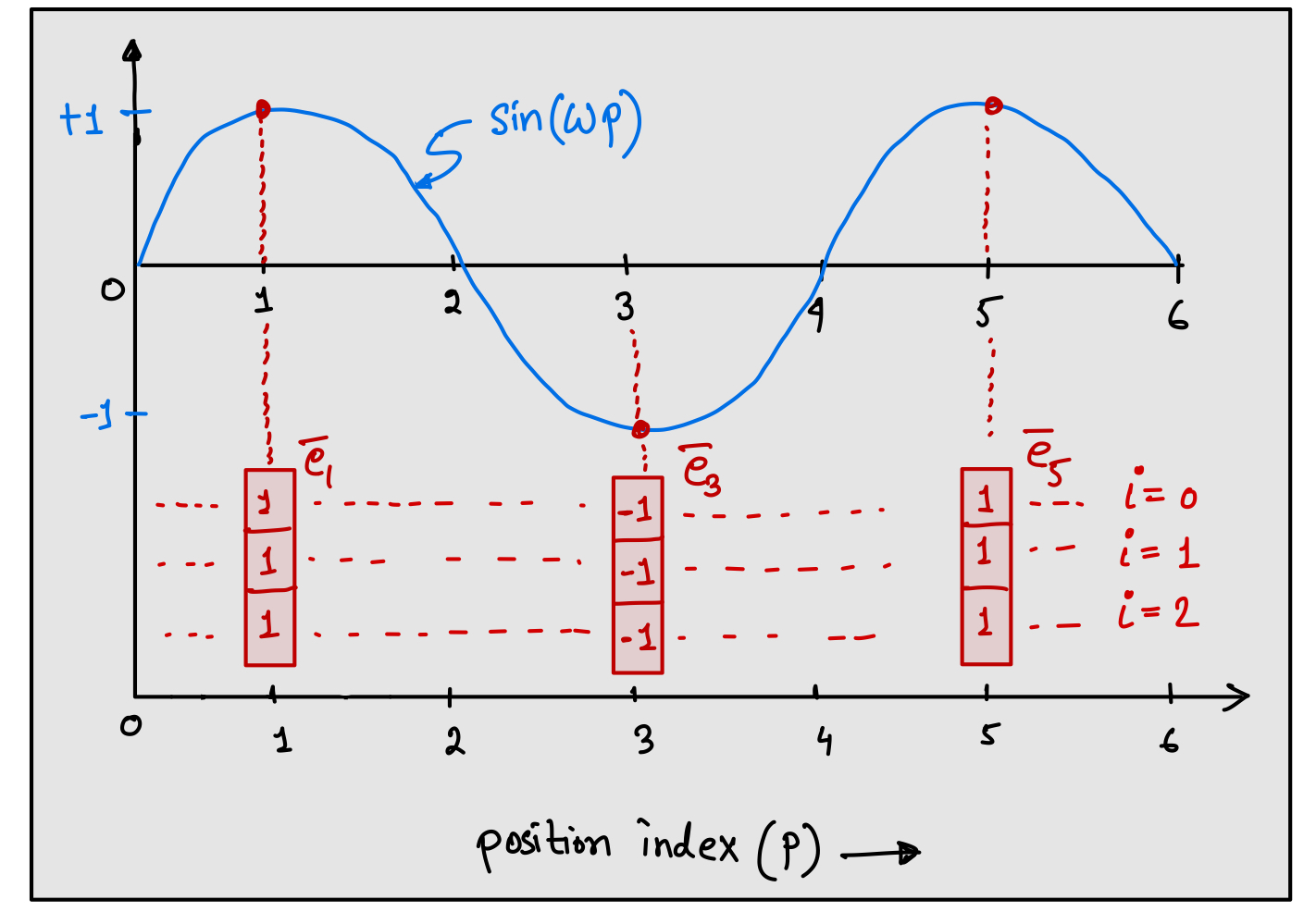
The family of sinusoidal functions such as sines and cosines satisfy one of the property that the values are bounded between [-1,1]. If you plot the values of sine as a function of position index, then the values won’t be unique after a full cycle as shown in the following figure.

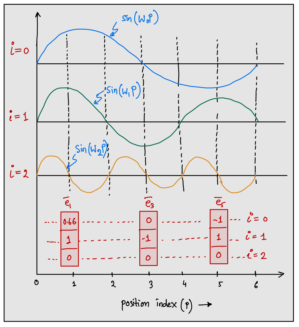
For example, if we use the sine function to represent the positional embedding then the values will be repeated for e1 and e5 which violates the property of positional embedding. The nature of the sine functions are always periodic, meaning their values are bound to repeat after a certain position. Since, we know that the positional embedding must be unique at all the positions, therefore to achieve uniqueness, we can use multiple sine functions with different frequency at different dimension index. Note that, in the figure, we can use different frequency $\omega$ for different dimension index $i$, instead of using the same $\omega$ for all the dimension indices. This allows us to create an embedding vector where each dimension values will be different (unlike the values shown in the figure), and if we can intelligently combine the sine functions, then we can acheive unique position embedding for all the positions.

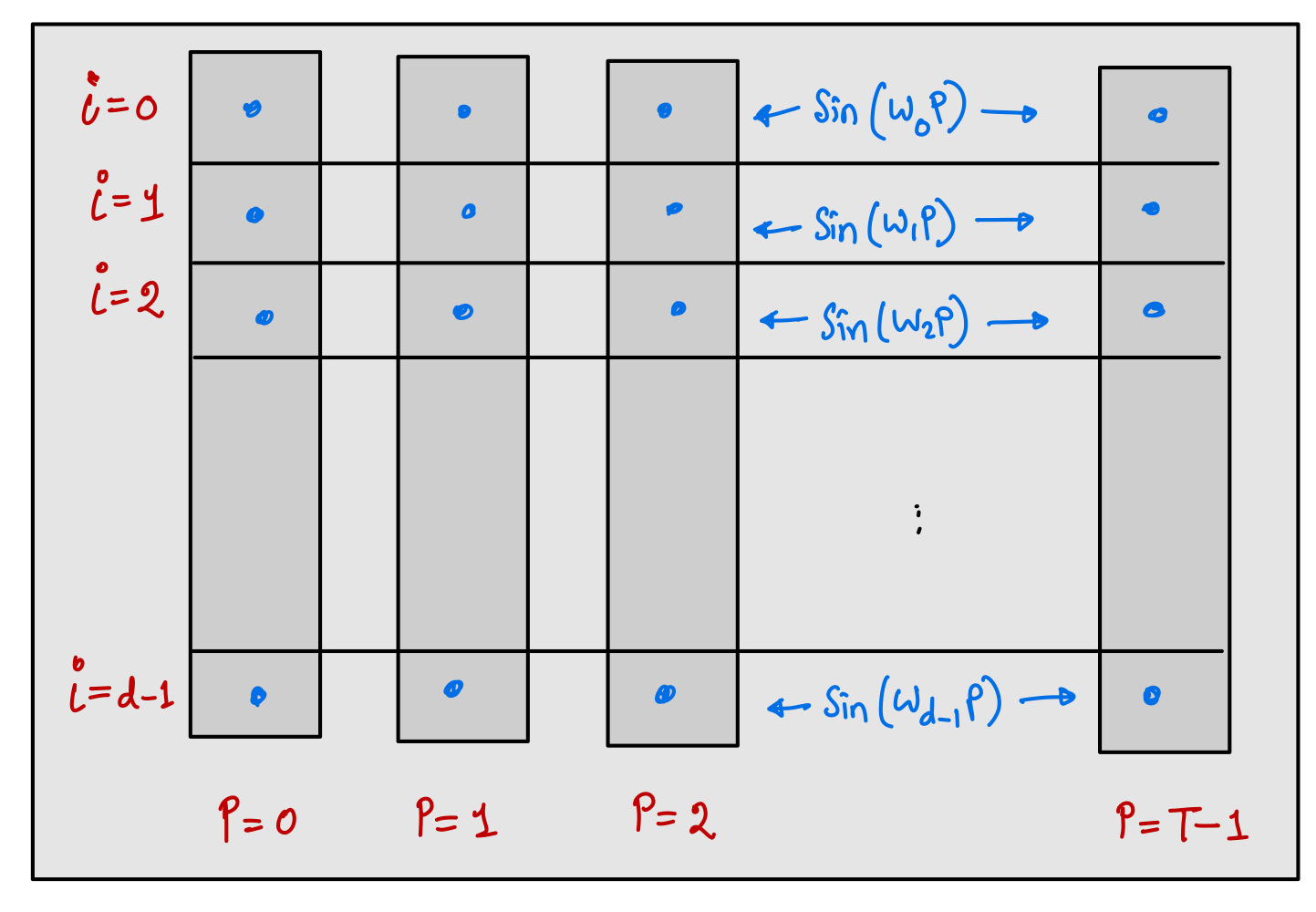
To get the unique positional embedding, we are going to vary the frequency at all the embedding components. From the above figure, it is clear that, the embedding vectors are unique. It means, the $i$-th component of the embedding vector at any position index $p$ will be obtained by taking the sine of $p$ with the frequency $\omega _ i$ as shown below:

[ \mathbf{e} _ p ^ i = \sin(\omega _ i \cdot p) \in \mathbb{R} \quad ; \mathbf{e} _ p = (\mathbf{e} _ p ^ i) _ {i = 0} ^ {i = d-1} \in \mathbb{R}^d ]

If we use the frequency values, $\omega _ 0, \omega _ 1, \dots, \omega _ {d-1}$ that are unique at all the dimension index (or component), then it is guaranteed that the positional embedding vector will be unique at all the positions.

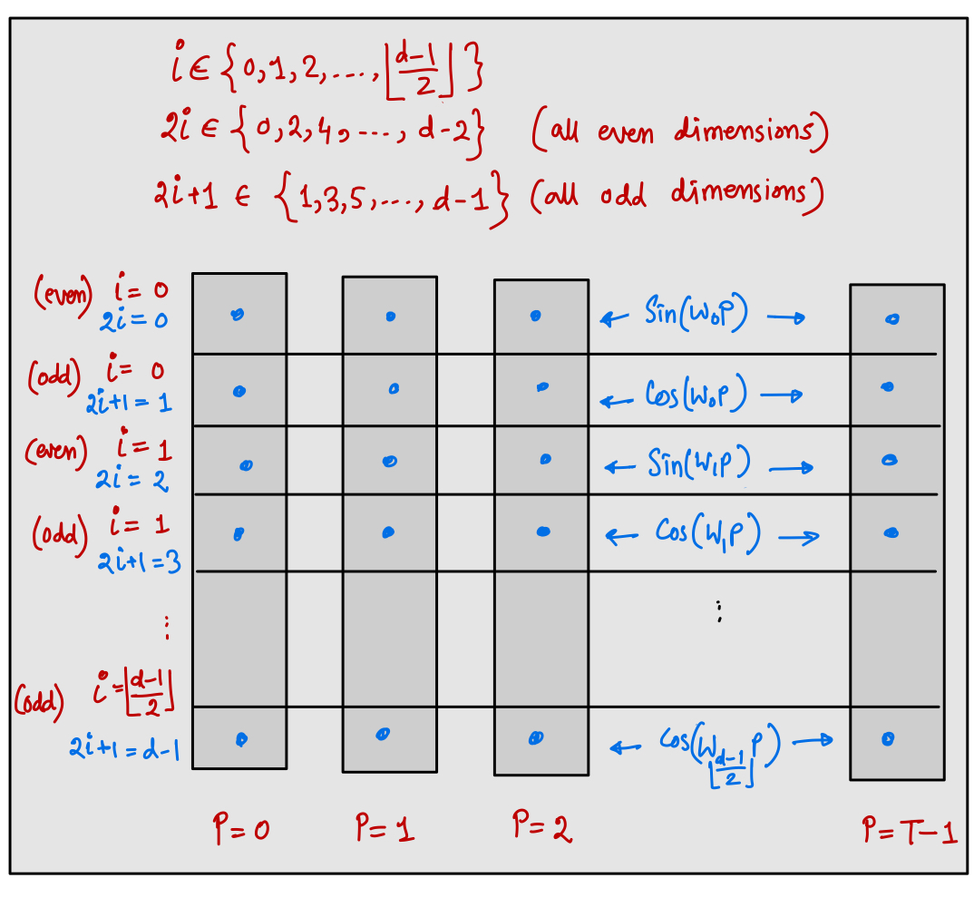
In the above figure, the process of obtaining the positional embedding values at all the positions and at all the dimension index is shown. Although, it was sufficient to use sine functions alone to obtain unique positional embedding, the author of Attention is All You Need paper used a mixture of sine and cosine functions. The idea is that, for even component of embedding vector, the sine function is used to obtain the values at all the positions, and for odd component of embedding vector, the cosine function is used to obtain the values as shown in the below figure:

The positional embedding vector for any position $p$ is given as:

[ \mathbf{e} _ p ^ {2i} = \sin(\omega _ i \cdot p) \in \mathbb{R} \quad ; \omega _ i = 1/10000^{2i/d} \quad; i \in {0, 1, \dots, \left\lfloor \frac{d-1}{2} \right\rfloor} ] [ \mathbf{e} _ p ^ {2i+1} = \cos(\omega _ i \cdot p) \in \mathbb{R} \quad ; \omega _ i = 1/10000^{2i/d} \quad; i \in {0, 1, \dots, \left\lfloor \frac{d-1}{2} \right\rfloor} ] [ \mathbf{e} _ p = (\mathbf{e} _ p ^ j) _ {j = 0} ^ {j = d-1} \in \mathbb{R}^d ]

Note that the positional embedding is function of position and it doesn’t matter, which word is present in that position. Since, there is no learnable parameter in the equation above, the positional embedding is not learnable. There are other variations of the above equation to make the implementation more straightforward. For example, instead of alternating usage of sine and cosine functions in even and odd positions, we can use the first half components as sine function and the rest half components as cosine function without violating any of the properties of positional embedding.

In LLM literature, there are numerous positional embedding that are in practice. Sinusoidal embeddings are not the only positional embedding that is used in LLM. GPT like LLMs do not even use the sinusoidal positional embedding which is non-learnable. Rather, the positional embedding is also learned from the training data during the pre-training stage.

Let’s now see the code of positional embedding layer in PyTorch.

import torch
import math

class PositionalEmbedding(torch.nn.Module):
    def __init__(self, embedding_dim: int, max_context_length: int):
        super(PositionalEmbedding, self).__init__()
        self.d = embedding_dim
        self.Tmax = max_context_length
        self.register_buffer(name="pos_emb", 
                             tensor=self.get_positional_embedding())
        
    def get_positional_embedding(self) -> torch.tensor:
        mid_index = int(math.ceil((self.d-1)/2)) # excluding mid_index
        position_tensor = torch.arange(0, self.Tmax).unsqueeze(1) # (Tmax, 1)
        pos_emb_list = []
        for i in range(mid_index):
            omega_i = 1 / (10000 ** (2 * i / self.d))
            pos_emb_list.append(torch.sin(position_tensor * omega_i))
            pos_emb_list.append(torch.cos(position_tensor * omega_i))
        
        pos_emb = torch.cat(pos_emb_list, dim=1)  # (Tmax, d)
        assert pos_emb.shape == (self.Tmax, self.d)
        return pos_emb
        
    def forward(self, x):
        """x.shape = (b, T)"""
        b, T = x.shape
        pos_emb = self.pos_emb[:T, :]  # (T, d)
        pos_emb = pos_emb.unsqueeze(0).expand(b, T, self.d)  # (b, T, d)
        return pos_emb

Note that the above code assumes that the dimension of embedding is always an even integer. Since the positional embedding needs to be stored as a state dictionary of the model (although it is not trainable!), I have used register_buffer to treat the pos_emb as a parameter of the model which is non-trainable. Moreover, the positional embedding is constant for all the input sequences in the batch (register_buffer would be covered in great detail in later sections). Therefore, the same positional embedding is expanded across all the input examples using expand method (similar to broadcasting!)

To test the code, we can pass a random input, as for positional embedding, the values of the input token IDs doesn’t matter. It is the number of token IDs ($T$) that matters for the computation.

pos_emb_layer = PositionalEmbedding(embedding_dim=4, max_context_length=6)
print(pos_emb_layer(x=torch.rand(size=(2,3)))) # (2, 3, 4)

tensor([[[ 0.0000,  1.0000,  0.0000,  1.0000],
         [ 0.8415,  0.5403,  0.0100,  0.9999],
         [ 0.9093, -0.4161,  0.0200,  0.9998]],

        [[ 0.0000,  1.0000,  0.0000,  1.0000],
         [ 0.8415,  0.5403,  0.0100,  0.9999],
         [ 0.9093, -0.4161,  0.0200,  0.9998]]])

Note that the positional embedding is same for both the examples in the batch as explained before.

1.2.4. Learnable Positional Embedding

2. Attention Layer

2.1. Motivation for Attention

2.2. Scaled Dot Product Attention

2.3. Causal Self Attention

2.4. Multi-head Self Attention

2.5. PyTorch’s Attention Layer

3. Transformer Layer

3.1. Layer Normalization

3.2. GELU and SoLU Activation

3.3. Feed Forward Layer

3.4. Residual Connection

4. GPT Model

4.1. Model Architecture

4.2. Generate Text

4.3. Greedy Decoding

4.4. Top-K Decoding

4.5. Effect of Temperature

What’s Next?

In next blog, I will cover …

Happy learning! 😃

Reference Books

• Sebastian Raschka, Build a Large Language Model (From Scratch)
• Aston Zhang, Dive into Deep Learning
• Daniel Jurafsky, Speech and Language Processing
• Huggingface tokenizers

Written by

Soumen Mondal (Email: 23m2157@iitb.ac.in), MS in AI and DS, CMInDS, IIT Bombay